1  Data overview

The analysis starts from a single consolidated file — CHOLERA_BAY 2018_2023.xlsx, a case line-list in which each row is one suspected cholera case. Before any trigger logic, we need to know what the file contains and how evenly it is populated.

1.1 What the line-list holds

	Field	Value
0	Rows (suspected cases)	32,826
1	Deaths	836
2	Date range (onset)	2018-01-02 → 2023-11-29
3	States	3
4	LGAs with ≥1 case	55
5	Wards with ≥1 case	731
6	Onset date present	100%

Each case carries an onset date (complete for every retained row — the backbone of any weekly signal), the reporting state, LGA and ward, an outcome (alive/dead), and patient age and sex. Oral cholera vaccine (OCV) fields exist but are sparsely filled. Crucially the line-list is suspected cases — it is not restricted to laboratory-confirmed cholera, which matters for how a trigger threshold should be read.

1.2 Cases by year and state

tab = (
    llp.pivot_table(index="year", columns="state", values="case", aggfunc="sum", fill_value=0)
    .reindex(columns=U.STATES)
)
fig, ax = plt.subplots(figsize=(10, 5))
bottom = np.zeros(len(tab))
for st in U.STATES:
    ax.bar(tab.index.astype(str), tab[st], bottom=bottom, label=st, color=U.STATE_COLORS[st])
    bottom += tab[st].values
for i, total in enumerate(tab.sum(axis=1)):
    ax.text(i, total + 200, f"{int(total):,}", ha="center", va="bottom", fontsize=10, fontweight="bold")
ax.set_ylabel("Suspected cases")
ax.set_title("Suspected cholera cases per year, by state (BAY, 2018–2023)")
ax.legend(title="State", ncol=3, loc="upper left")
ax.margins(y=0.12)
plt.tight_layout()
plt.show()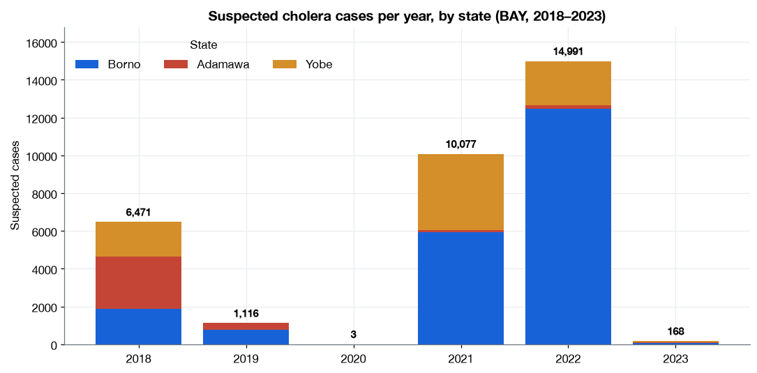

Figure 1.1: Suspected cholera cases per year, by BAY state. Three large outbreak years (2018, 2021, 2022) dominate; 2020 is almost empty.

The burden is dominated by three years — 2018, 2021 and 2022 — with Borno carrying most cases in the largest years. 2019 and 2023 are thin, and 2020 is effectively absent. The next chapter shows the 2020 gap is a reporting failure, not a true absence of cholera.

1.3 Case-fatality by year

summ = (
    ll.groupby("year")
    .agg(cases=("case", "sum"), deaths=("death", "sum"))
    .assign(cfr_pct=lambda d: (100 * d["deaths"] / d["cases"]).round(2))
    .reset_index()
)
total = pd.DataFrame(
    {
        "year": ["All"],
        "cases": [summ["cases"].sum()],
        "deaths": [summ["deaths"].sum()],
        "cfr_pct": [round(100 * summ["deaths"].sum() / summ["cases"].sum(), 2)],
    }
)
out = pd.concat([summ, total], ignore_index=True)
out.columns = ["Year", "Cases", "Deaths", "CFR (%)"]
out.style.hide(axis="index").format({"Cases": "{:,}", "Deaths": "{:,}"})

Table 1.1: Cases, deaths and case-fatality ratio (CFR) by year.

Year	Cases	Deaths	CFR (%)
2018	6,471	234	3.620000
2019	1,116	3	0.270000
2020	3	0	0.000000
2021	10,077	237	2.350000
2022	14,991	358	2.390000
2023	168	4	2.380000
All	32,826	836	2.550000

Overall CFR sits around 2.5%, above the <1% target for well-managed cholera response and consistent with outbreaks in hard-to-reach conflict-affected areas. The near-zero 2019 CFR (0.3%) is an artefact of that year’s sparse reporting rather than unusually mild disease.

1.4 Geographic spread

g = (
    llp.groupby("state")
    .agg(
        cases=("case", "sum"),
        deaths=("death", "sum"),
        lgas=("ADM2_PCODE", "nunique"),
    )
    .reindex(U.STATES)
    .reset_index()
)
g["cfr_pct"] = (100 * g["deaths"] / g["cases"]).round(2)
g.columns = ["State", "Cases", "Deaths", "Affected LGAs", "CFR (%)"]
g.style.hide(axis="index").format({"Cases": "{:,}", "Deaths": "{:,}"})

Table 1.2: Cases, deaths and number of affected LGAs by state.

State	Cases	Deaths	Affected LGAs	CFR (%)
Borno	21,132	564	26	2.670000
Adamawa	3,459	52	13	1.500000
Yobe	8,235	220	17	2.670000

Cases reach dozens of LGAs, but as Epidemiology shows, a small number of LGAs account for most of the burden — which is what makes an LGA-level trigger plausible.