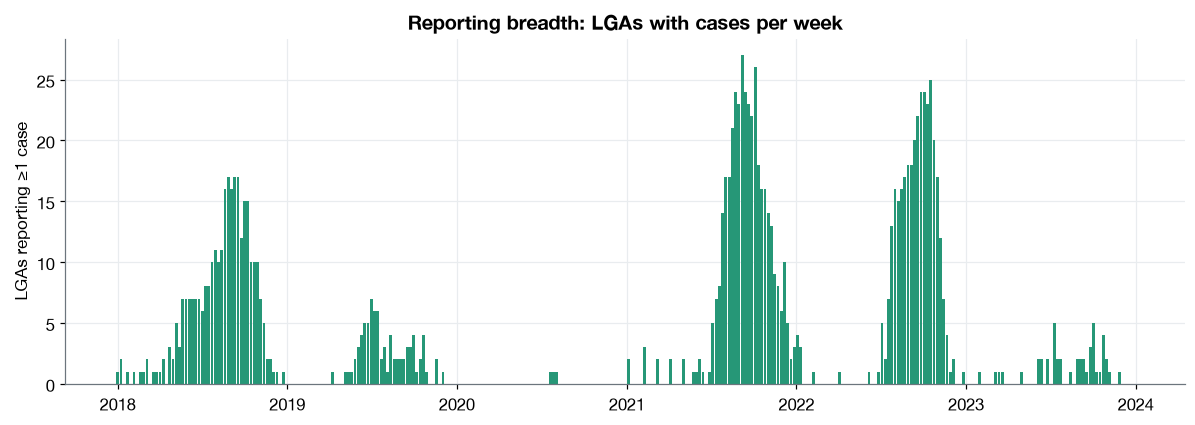
A trigger is only as good as the data feeding it. This chapter asks whether the line-list reports consistently enough to calibrate percentile thresholds, and what the gaps do to those thresholds.
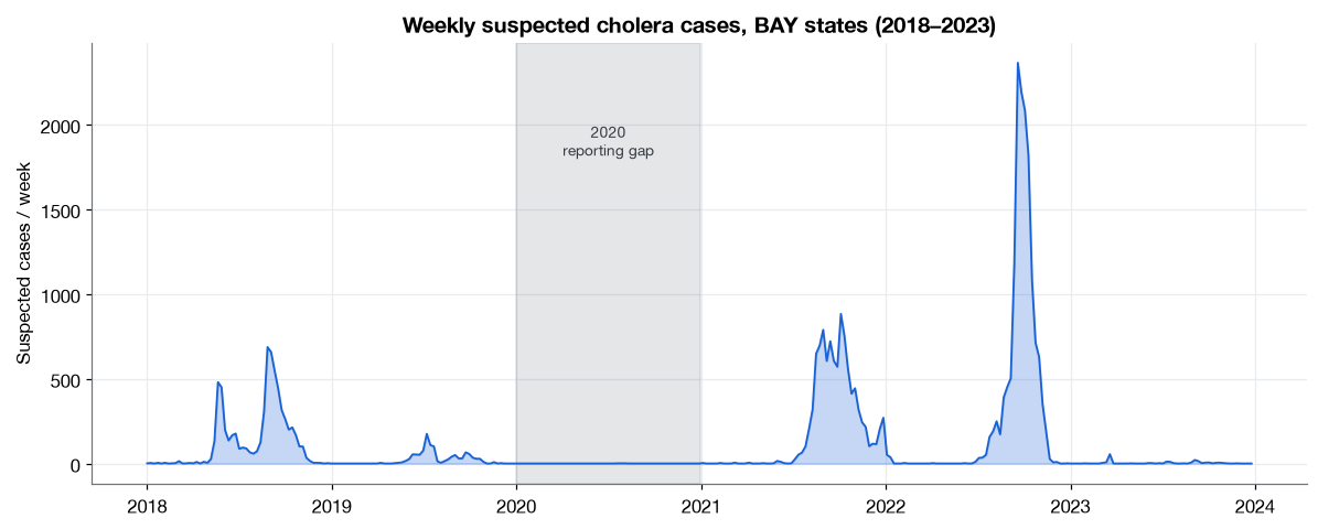
Figure 2.1: Suspected cases per week across all three BAY states. Grey band marks the 2020 reporting collapse.
The series is spiky and seasonal, with sharp peaks in the outbreak years and long near-zero stretches between them. The 2020 stretch is not a genuine lull.
Table 2.1: Reporting depth by year: cases, active weeks, and the number of distinct LGAs reporting.
Year
Cases
Weeks with ≥1 case
LGAs reporting
2018
6,471
46 / 52
37
2019
1,116
29 / 52
13
2020
3
3 / 52
1
2021
10,077
36 / 52
41
2022
14,991
31 / 52
34
2023
168
24 / 52
18
2.2 Gap identification
Three years fall short of usable reporting:
2020 — effectively empty (3 cases). WHO and partner reporting confirm cholera transmission across BAY states in 2020; the line-list simply does not capture it. This is a data gap.
2019 — thin (≈1,100 cases, near-zero deaths). Plausibly a genuinely quieter year, but the 0.3% CFR hints at under-capture too.
2023 — partial (168 cases, ends late November). The file was compiled mid-outbreak-cycle; 2023 is truncated, not complete.
2.2.1 What this means for zero-filling
We build the LGA × week panel by zero-filling every week an LGA reports nothing. That is the right choice for a seasonal signal (most weeks genuinely have no cholera), but it is the wrong choice for a reporting-gap year: zero-filling 2020 asserts “no cholera” when the truth is “no data”. Percentile thresholds computed over a window that includes 2020 are therefore biased downward.
2.3 Impact on percentile baselines
How much does including the gap years move the threshold? The candidate trigger keys off the 99th percentile of weekly cases. Below we recompute that percentile for each state over three baseline choices.
Show code
def p99_by_state(df):return {st: np.percentile(df[df["state"] == st]["cases"], 99) for st in U.STATES}full = p99_by_state(sw)no2020 = p99_by_state(sw[sw["week"].dt.year !=2020])outbreak = p99_by_state(sw[sw["week"].dt.year.isin([2018, 2021, 2022])])imp = pd.DataFrame( {"State": U.STATES,"All years (2018–23)": [round(full[s]) for s in U.STATES],"Excl. 2020": [round(no2020[s]) for s in U.STATES],"Outbreak yrs only": [round(outbreak[s]) for s in U.STATES], })imp.style.hide(axis="index")
Table 2.2: 99th-percentile weekly cases per state under three baseline windows. Including gap years pulls thresholds down.
State
All years (2018–23)
Excl. 2020
Outbreak yrs only
Borno
1640
1769
1882
Adamawa
131
152
293
Yobe
347
350
355
The effect is modest at the state level here (the outbreak weeks that set the 99th percentile survive in every window), but it grows for shorter rolling windows and for per-LGA thresholds, where a single gap year is a larger share of the baseline. The practical rule matches the DRC analysis’s conclusion.
Recommendations for calibration
Exclude 2020 from any baseline pool — it is missing data, not a quiet year.
Treat 2019 and 2023 as partial; prefer a baseline anchored on the well-reported outbreak years (2018, 2021, 2022) when setting thresholds.
Prefer an expanding / multi-year baseline over a short rolling window, so no single bad year dominates the threshold.
Before operational use, confirm a minimum-reporting guard (e.g. require a minimum number of reporting LGAs in a week) so a reporting rebound isn’t mistaken for an outbreak.
2.4 Timeliness — the binding constraint
This retrospective file cannot answer the question that matters most for AA: how quickly do these records arrive? A trigger needs case data within days-to-weeks of onset. The earlier BAY exploration flagged timeliness as the primary blocker, and nothing in this file resolves it. Every result that follows is retrospective and assumes data that, in production, would need to arrive fast enough to act on.